Introduction
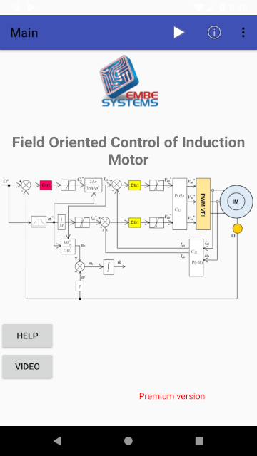
This application allows to simulate the Field Oriented Control (FOC, or vector control) of induction machines, in speed and current control and to visualize curves and values.
It allows to choose between 4 types of Field Oriented Control:
IRFOC : Indirect Rotor Field Oriented Control
DRFOC : Direct Rotor Field Oriented Control
ISFOC : Indirect Stator Field Oriented Control
DSFOC : Direct Stator Field Oriented Control
It is possible to choose between a current control, with only Ids and Iqs PI currents controllers, or to add an external speed control loop (IP anti-windup).
We also visualize on an alpha-beta stator fixed frame, the dq rotating frame with the stator and rotor flux vectors as well as the current Is and its components Ids and Iqs.
An animation based on simulation time allows to better understand the interactions of these variables and the behavior of the control on the motor.
Thank you for considering a 5-star vote for this app, which will allow its wide dissemination to the community of students and teachers of Electrical Engineering.
If you have any concern, please let me know before voting, by email:
I could certainly provide explanations, without getting a vote below 5 stars.
I am a teacher-researcher in EE: Researchgate Profil
Thank you for encouraging the development of this kind of apps, by contributing through an in-app purchase of the Premium offer, for 3.2.
Summary
The FOC Field Oriented Control of IM App helps students and teachers to study and understand the vector control of the Induction Machine and its transient behavior.
Several events can be applied during the simulation, such as changes in load torque at different times, reference speeds and reference currents Idsref and Iqsref, as well as resistive parameter variations.
Simulations can be shared and exported to other apps (Gmail, photos, Excel sheets, documents).
Main characteristics:
Simulation of vector control of the Induction machine (IM), in speed and current control
Curves of Idsref, Iqsref, Ids, Iqs currents and Vdsref, Vqsref voltages, electromagnetic torque, speed, rotor and stator flux in alpha-beta, as a function of time and in steady state
Application of Clarke and Park transformations to three-phase variables (voltages and currents)
Field Oriented Control: IRFOC, DRFOC, ISFOC, DSFOC
Current control (Ids, Iqs) and speed control
Ideal inverter (sinusoidal voltage) or 2-level PWM (Pulse Width Modulation)
Change motor parameters and save them in local files
Apply several load torque events, speed reference... in the simulation
Simulation parameters (final time, step time...)
Displays the curves by splitting the window into 2 graphs, with zoom and display of values on the curve point
Premium Version:
Additional events (speed reference Wmref, Idsref, Iqsref, stator and rotor resistance) instead of only load torque events
Display an infinity of curves on the 2 graphs with selection of the color, the top/bottom position and the primary or secondary Y-axis of the graph. It is limited to 3 curves in the basic version
Load previously saved configuration, and also share them by email
Export data: graph images, graph data (xls/csv), machine parameters
And of course you help the developer, who is a teacher and researcher in electrical engineering, in his approach to develop educational apps
Navigation
Through 7 screens or views, you access the different configurations and parts of the application.
You navigate by sliding (swipe) the different views laterally or
By selecting the corresponding view from the menu
You can also, from the home screen ,
click on the part of the diagram that represents the configuration or the view in question.
Simulation: Click on current controller loops (rouge) to access simulation parameters.
Curves: Click on Ias, Ibs currents (violet) to display curves.
Results: Swipe views or from the menu to view the results.
Flux vectors: Swipe views or from the menu to display the animated alpha-beta frame.
Events: Click on the reference speed (green) to access simulation events.
Parameters : Click on Induction motor (blue) to change parameters.
Simulation
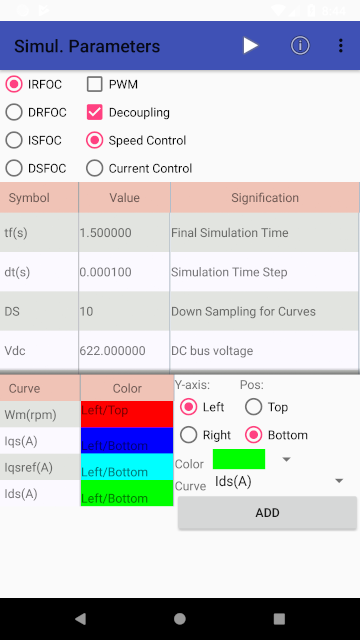
The "Simul. Parameters" view allows you to choose the different simulation options to apply.
By clicking on the control loops (red) of the home screen diagram,
we can choose between 4 types of vector control:
IRFOC : Indirect Rotor Field Oriented Control
DRFOC : Direct Rotor Field Oriented Control
ISFOC : Indirect Stator Field Oriented Control
DSFOC : Direct Stator Field Oriented Control
It is possible to choose between current control, with PI control of Ids and Iqs currents only, or add an external loop for speed control (IP anti-windup) _by default_.
One can also choose whether to use an ideal inverter (which sends sinusoidal voltages) or a 2-levels one controlled in PWM (Pulse Width Modulation).
Other numeric parameters are grouped in a table. These parameters can be changed by a long press on the row of the table.
We choose the simulation time (tf), the calculation step (dt= 1.e-4s)
The DS (down sampling) allows you to save only one point every DS (10 for example).
This is particularly useful when the time constants of the IM are small or with the PWM and we must decrease the computation step but we do not want to have curves with many points that would make their display and handling heavy.
For a PWM of 10 kHz (100 us), a computation step of 1.e-5s at the most is necessary and therefore DS will be set to 100 instead of 10.
Decoupling allows to introduce or not the static decoupling terms at the output of the current controllers Ids and Iqs.
For the curves, we must choose the color then the position (in the top or bottom graph) and if it uses the main Y-axis (left) or the secondary Y-axis (right). Finally, we add the curve to the left panel.
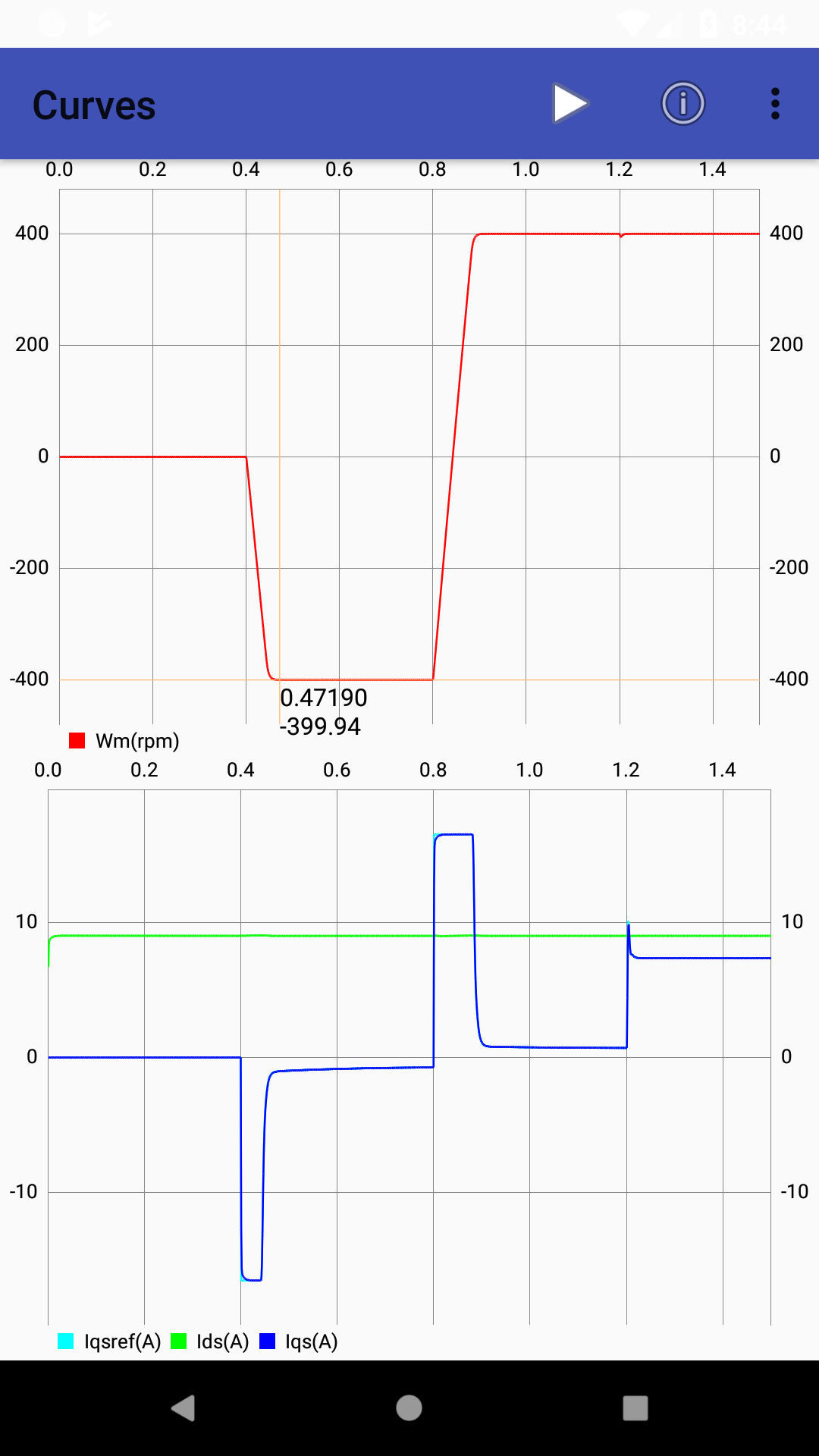
Curves
The "Curves" view allows you to see the instantaneous curves of the motor variables.
It is also accessed by launching the simulation using the Run icon
The results are then displayed:
We can choose in the Simulation view, the curves to be displayed.
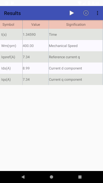
Results
The "Results" view is used to display the numerical values of the quantities for a given point.
However, if we click on the curves, a point appears and the calculation is done again for this point.
It is better to navigate to the Results view, with the menu to avoid changing this point, by dragging the view laterally.
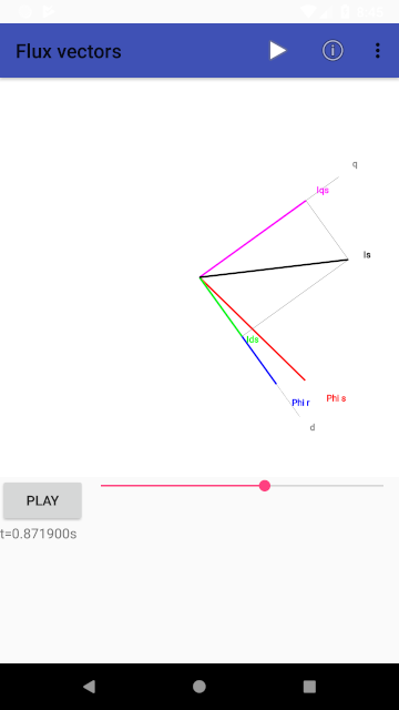
Flux Vectors
The "Flux Vectors" view is used to animate the flux vectors Phi_s and Phi_r on an alpha-beta stator fixed frame and thus show how the d-axis carries the entire rotor flux (in IRFOC and DRFOC) or the stator flux (in ISFOC and DSFOC).
We also display the current Is and its 2 components Ids and Iqs.
The Play / Stop button allows the animation and the slider permits to navigate on the entire duration of the simulation.
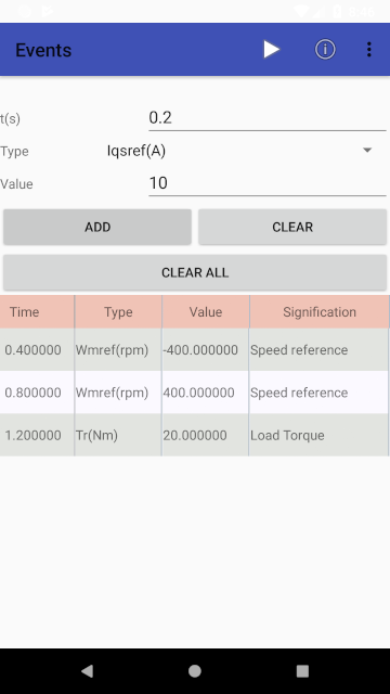
Events
The "Events" view allows you to choose the different events to apply.
A long press on a row of the added events table allows you to change the application time of the event and its value.
Several events can follow each other, for example, Wmref=-400 rpm at t=0.4s, then Wmref=+400 rpm at t=0.8s, then Cr=20 Nm at t=1.2s.
Other types of events can be added such as Iqsref, Idsref, variation of the stator and rotor resistance (Premium option).
IM Parameters
The "IM Parameters" view allows to choose the different electromagnetic and mechanical parameters of the induction motor as well as the parameters of the model used for the control.
The menu also allows you to choose IM Parameter saving.
The chosen name must have a .focfg extension to be recognized when receiving such a file sent via Gmail or other programs.
You can also choose Loading Settings from backups, this is a Premium option.
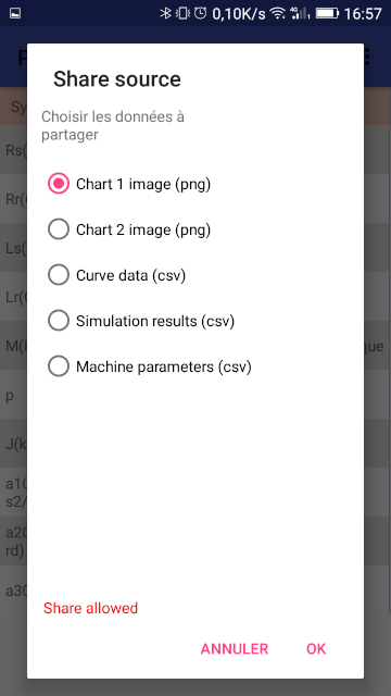
The Share menu (Premium) allows you to send the IM parameters file to other devices / users, for example via Gmail.
The Exports menu (Premium) is extremely useful and allows you to send the curve image to other apps, such as File Manager, Viber or Gmail.
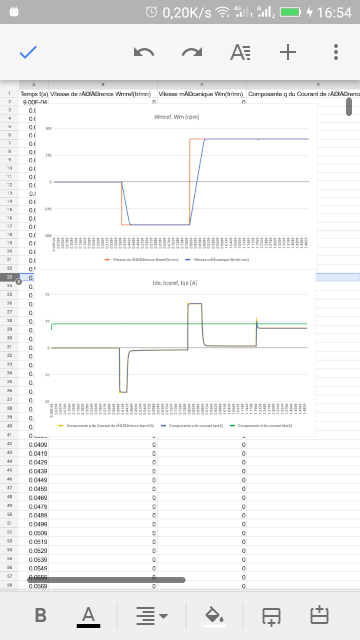
For data, you can send the data to the file manager to save a file, data .csv for example, which you can then send by email or open with Excel or Sheets app.
This very interesting option makes it possible to use the results of the simulation later using the generated .csv file.